Additional Mathematics notes, chapter 5
Probability Distribution
Textbook Additional Mathematics Form 5 (DLP), pages 140–187
What this chapter covers
- Recognise a random variable, and tell discrete from continuous random variables (5.1)
- Build and use the probability distribution of a discrete random variable, and show that the probabilities add up to 1 (5.1)
- Recognise Bernoulli trials and a binomial distribution X ~ B(n, p), and find P(X = r) (5.2)
- Find the mean np, variance npq and standard deviation of a binomial distribution, and solve problems (5.2)
- Describe the normal distribution X ~ N(μ, σ²) and its bell-shaped graph (5.3)
- Standardise a normal variable with Z = (X − μ)/σ, find probabilities from the standard normal table, and find a value of X from a given probability (5.3)
5.1Random variable
A random variable is a variable with numeric values that depend on chance. It is written with a capital letter such as X, and its values with small letters such as r. Example: X = number of wins in two matches, X = {0, 1, 2}.
| Type | Values | Example |
|---|---|---|
| Discrete random variable | Countable, usually 0 and positive whole numbers: X = {r : r = 0, 1, 2, 3} | Number of heads in 3 tosses |
| Continuous random variable | Any value in an interval: Y = {y : a < y < b} | Time spent waiting at a bus stop, height of pupils |
Example 2 (textbook p. 144): discrete or continuous?
(a) A fair dice is thrown 3 times. X = number of 4s. X = {0, 1, 2, 3}, a discrete random variable because the values can be counted.(b) X = waiting time between 5 and 55 minutes. X = {x : 5 < x < 55}, a continuous random variable because the values lie in an interval.
A number of items is discrete. A measurement (time, mass, height) is continuous, even if you round it when you record it.
Probability distribution of a discrete random variable
If X takes the values r₁, r₂, …, rₙ, then every P(X = rᵢ) is between 0 and 1 and the total probability is ΣP(X = rᵢ) = 1.
A distribution can be shown as a tree diagram, a table or a bar graph. Add up the probabilities of all the branches that give the same value of X.
Worked example: a spinner with 1/4 of it shaded, spun 3 times
X = number of times the pointer stops on the shaded part. P(shaded) = ¼, P(not shaded) = ¾.P(X = 0) = (¾)³ = 27/64. P(X = 1) = 3 × ¼ × (¾)² = 27/64. P(X = 2) = 3 × (¼)² × ¾ = 9/64. P(X = 3) = (¼)³ = 1/64.
| r | 0 | 1 | 2 | 3 |
|---|---|---|---|---|
| P(X = r) | 27/64 | 27/64 | 9/64 | 1/64 |
Three branches give X = 1, so multiply the single-branch probability by 3. This "number of orders" is the idea behind the binomial formula.
A discrete random variable has P(X = r) = k(r + 1) for r = 0, 1, 2, 3. Find k.
Show answerHide answer
k(1 + 2 + 3 + 4) = 1, so 10k = 1 and k = 1/10.
5.2Binomial distribution
Bernoulli trials
A Bernoulli trial has only two outcomes, "success" with probability p and "failure" with probability q = 1 − p. A binomial distribution counts the successes in n trials, X ~ B(n, p), when the trials are:
- fixed in number, n;
- independent, each with only two outcomes;
- the same probability of success p every time.
Drawing from a small group without putting items back changes p each time, so it is not binomial. A survey of a very large population is treated as binomial.
The binomial probability function
P(X = r) = nCr pr qn−r, r = 0, 1, 2, …, n. Here r = number of successes, p = probability of success, q = 1 − p.
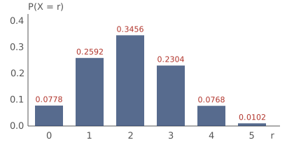
Example: X ~ B(6, 0.3), find P(X = 2)
P(X = 2) = 6C2(0.3)²(0.7)⁴ = 15 × 0.09 × 0.2401 = 0.3241"At least one" is easier as 1 − P(X = 0). "Not more than 2" means P(X ≤ 2) = P(0) + P(1) + P(2).
Mean, variance and standard deviation
| Quantity | Formula |
|---|---|
| Mean | μ = np |
| Variance | σ² = npq |
| Standard deviation | σ = √(npq) |
Example 11 (textbook p. 162) style: 95% have a driving licence, 160 people chosen
n = 160, p = 0.95, q = 0.05. Mean = 160 × 0.95 = 152. Variance = 160 × 0.95 × 0.05 = 7.6. Standard deviation = √7.6 = 2.76.Example 12 (textbook p. 163): how many must be checked?
12% of cakes weigh under 1 kg. Find the least n so that P(X ≥ 1) > 0.85.1 − (0.88)ⁿ > 0.85, so (0.88)ⁿ < 0.15. Take logs: n log 0.88 < log 0.15, and dividing by the negative log 0.88 reverses the sign: n > log 0.15 / log 0.88 = 14.84. The least n is 15.
Dividing both sides by log 0.88 (a negative number) flips the inequality sign. Round n up to the next whole number.
X ~ B(150, 0.2). Find the mean and the standard deviation.
Show answerHide answer
Mean = 150 × 0.2 = 30. Variance = 150 × 0.2 × 0.8 = 24. Standard deviation = √24 = 4.90.
5.3Normal distribution
A normal distribution X ~ N(μ, σ²) is a distribution of a continuous random variable with mean μ and standard deviation σ. Its graph is bell-shaped and symmetrical about the line x = μ.
- The total area under the curve is 1, so P(−∞ < X < ∞) = 1. The area is the probability.
- Half of the area (0.5) is on each side of μ.
- A larger μ moves the curve to the right. A larger σ makes the curve wider and lower.
- The curve has its highest point at x = μ, and both ends go on indefinitely without touching the x-axis.
- For a continuous variable P(X = a) = 0, so P(X < a) and P(X ≤ a) are equal.
A binomial distribution with a large n is hard to work out, so it can be estimated by a normal distribution when np > 10 and n(1 − p) > 10.
For a normal distribution, about 68% of the data lies within 1 standard deviation of the mean, 95% within 2 and 99.8% within 3.
Standard normal distribution
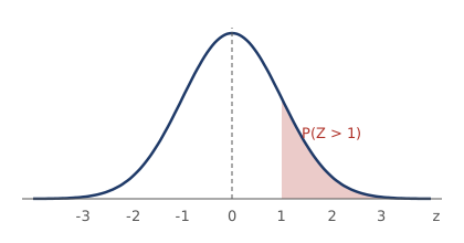
The standard normal distribution is Z ~ N(0, 1), with mean 0 and standard deviation 1. Any normal variable is standardised by Z = (X − μ) / σ.
| Probability wanted | How to find it |
|---|---|
| P(Z > z) for z ≥ 0 (the textbook table gives this right-tail area) | Read it straight off the table |
| P(Z < −z) | Same as P(Z > z), by symmetry |
| P(Z < z) | 1 − P(Z > z) |
| P(a < Z < b) | 1 − P(Z < a) − P(Z > b), or P(Z > a) − P(Z > b) when 0 < a < b |
Example: heights X ~ N(165, 6²) cm
P(X > 171): Z = (171 − 165)/6 = 1, so P(Z > 1) = 0.1587 from the table.P(159 < X < 177): Z from −1 to 2, so P = 1 − 0.1587 − 0.0228 = 0.8185.
Finding a value of X from a probability
Example: the top 10% of marks, X ~ N(62, 10²)
P(Z > k) = 0.1, and the table gives k ≈ 1.28 (1.282 on a calculator). X = μ + kσ = 62 + 1.282 × 10 = 74.8 marks.Draw a quick sketch and shade the area. It shows whether to subtract from 1, and whether the z-value is positive or negative.
Using σ² instead of σ. In N(50, 16) the standard deviation is √16 = 4, not 16.
Law of large numbers
The law of large numbers: the larger the sample, the smaller the random variation, so the experimental mean gets closer to the theoretical mean (textbook p. 169). Tossing a coin 10 times might give 7 heads, but 10 000 tosses give a number of heads close to 5 000.
X ~ N(60, 25). Find P(X > 70).
Show answerHide answer
σ = 5. Z = (70 − 60)/5 = 2. P(Z > 2) = 0.0228 from the table.