Mathematics notes, chapter 12

Measures of Central Tendencies

Textbook Mathematics Form 2 (DLP), pages 244–275

What this chapter covers

Determine the mode, mean and median of a set of ungrouped data, including data in frequency tables and data representations (12.1.1)
Explain the effect of an extreme value, and of changing every value uniformly or non-uniformly, on the mode, mean and median (12.1.2)
Collect, construct and interpret frequency tables for grouped data (12.1.3)
Determine the modal class and the mean of a set of grouped data using midpoints (12.1.4)
Choose and justify the most appropriate measure of central tendency, including for data with extreme values (12.1.5)
Determine the mode, mean and median from data representations (12.1.6)
Use measures of central tendency, and the range, to make predictions, form arguments and draw conclusions (12.1.7)

A measure of central tendency describes a whole set of data with one value that shows where the data is centred. Shops, teachers and sports coaches use it to compare groups and to make decisions. Three measures are used: the mode, the median and the mean.

Remember the three like this. Mode = most often. Median = in the middle (after arranging in order). Mean = the "fair share" or average (total ÷ number of values).

English	Bahasa Melayu
measure of central tendency	sukatan kecenderungan memusat
mode, median, mean	mod, median, min
extreme value	nilai ekstrem
frequency table	jadual kekerapan
modal class, midpoint	kelas mod, titik tengah

12.1.1Mode, mean and median of ungrouped data

Mode

The mode is the value with the highest frequency, the one that appears most often. A set of data can have one mode, two modes (equal highest frequencies) or no mode (every value appears equally often).

Example 1 (textbook p. 247): state the mode

(a) 4, 5, 2, 3, 4, 4, 5 → 4 appears 3 times, so the mode is 4.
(b) M, N, L, M, L, P, L, L, P → L appears 4 times, so the mode is L.
(c) Coffee, Tea, Coffee, Coffee, Milk, Tea, Milk, Tea → Coffee and Tea both appear 3 times: the modes are Coffee and Tea.
(d) 2, 4, 6, 8, 10 → no value is repeated: no mode.

The mode is the value that appears most often, not its frequency. In (a) the mode is 4, not 3.

Median

The median is the middle value when the data is arranged in ascending or descending order. If the number of values is odd, take the value in the middle. If it is even, take the average of the two middle values.

Example 3 (textbook p. 249): goals scored in 10 games

1, 5, 1, 1, 4, 2, 5, 1, 4, 4
Arrange in order: 1, 1, 1, 1, 2, 4, 4, 4, 5, 5
There are 10 values (even), so the median is the average of the 5th and 6th values: (2 + 4) ÷ 2 = 3.

Always arrange the data in order first. The middle of the list as it was written is not the median.

Median from a frequency table

When the data is in a frequency table, work out the positions of the values by adding up the frequencies. Let n be the total frequency.

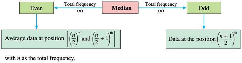
Flow chart. Total frequency n even: average of the data at positions n over 2 and n over 2 plus 1. Total frequency n odd: data at position (n plus 1) over 2. — Median by position (textbook p. 250).

Figure: Mathematics Form 2 (DLP) textbook, p. 250.

Example 5 (textbook p. 250): 12 groups, frequency table

Time (minutes)	10	20	30	40
Frequency	2	4	5	1
Position of data	1–2	3–6	7–11	12

n = 12 (even). The median is the average of the 6th and 7th values.
The 6th value is 20 and the 7th value is 30, so the median = (20 + 30) ÷ 2 = 25.

Median from a dot plot

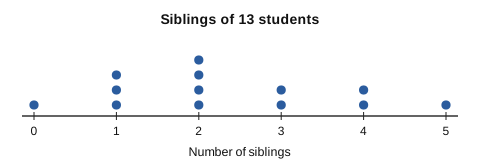
Dot plot of the number of siblings of 13 students. 0 siblings: 1 dot, 1: 3 dots, 2: 4 dots, 3: 2 dots, 4: 2 dots, 5: 1 dot. — 13 students: n is odd, so the median is at the (13 + 1) ÷ 2 = 7th position. Counting dots from the left: 1, 4, 8, so the 7th value is 2. Median = 2 siblings.

Mean

Mean = the sum of all the values ÷ the number of values. For a frequency table, mean = (sum of value × frequency) ÷ total frequency.

Example 7 (textbook p. 252): jogathon collection of five classes

RM373.50, RM424.00, RM363.00, RM485.15, RM355.10
Mean = RM2 000.75 ÷ 5 = RM400.15

Example 9 (textbook p. 253): mean from a frequency table

Internet hours: 1, 2, 3, 4, 5 with frequencies 2, 6, 11, 7, 9
Add a row of value × frequency: 2, 12, 33, 28, 45, which total 120. The frequencies total 35.
Mean = 120 ÷ 35 = 3.43 hours

Another frequency table: books borrowed by 24 students

Books	1	2	3	4
Frequency	4	8	6	6
Books × frequency	4	16	18	24

Mode = 2 books (highest frequency 8).
Median: n = 24, so average of the 12th and 13th values. The positions are 1–4, 5–12, 13–18, 19–24. The 12th is 2 and the 13th is 3, so the median = 2.5.
Mean = (4 + 16 + 18 + 24) ÷ 24 = 62 ÷ 24 = 2.58 (2 d.p.).

In a frequency table, the mean is not the sum of the values 1 + 2 + 3 + 4 divided by 4. Each value must be multiplied by how often it occurs.

Find the mode, median and mean of 8, 3, 6, 3, 10, 3, 9, 6.

Show answerHide answer

Mode = 3 (appears 3 times).
Ordered: 3, 3, 3, 6, 6, 8, 9, 10. Median = (6 + 6) ÷ 2 = 6.
Mean = 48 ÷ 8 = 6.

Extreme values

An extreme value is a value that is much smaller or much larger than the other values in the set.

Dot plot of the time in minutes taken by 7 students: 5, 6, 7, 7, 8, 9 and one far-away dot at 20 marked extreme value. — Example 10 (textbook p. 253). 20 is an extreme value: it is far larger than the others.

Example 12 (textbook p. 254): the impact of an extreme value

Pocket money of 5 students: RM3, RM4, RM4, RM6, RM8. Mode = RM4, median = RM4, mean = RM25 ÷ 5 = RM5.
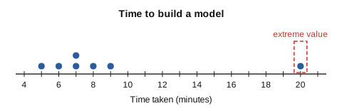
Replace RM8 with RM32 (an extreme value): mode = RM4, median = RM4, mean = RM49 ÷ 5 = RM9.80.
The mean rose by RM4.80, but the mode and the median did not change.

An extreme value pulls the mean towards it. The median and mode are not affected by it.

12.1.2The effect of changing the data

The data is changed	Mode, median and mean
Uniformly: the same number is added, subtracted, multiplied or divided on every value	All three change in the same way
Non-uniformly: values are changed by different amounts	All three change in no fixed pattern; work them out again

Example 13 (textbook p. 255): prices of 5 items

RM1, RM2, RM3, RM3, RM6: mean = RM3, median = RM3, mode = RM3.
(i) Each price rises by RM2: RM3, RM4, RM5, RM5, RM8 gives mean = RM5, median = RM5, mode = RM5. Each measure also went up by RM2.
(ii) Each price is multiplied by 3: RM3, RM6, RM9, RM9, RM18 gives mean = RM9, median = RM9, mode = RM9. Each measure is also multiplied by 3.

Example 14 (textbook p. 256): non-uniform change

Scores 3, 6, 6: mean = 5, median = 6, mode = 6. Add 1, 2 and 3 to the first, second and third score: 4, 8, 9.
New mean = 21 ÷ 3 = 7 and new median = 8, and there is no mode. The mean and median each went up by 2 but the mode disappeared, so the three measures did not change in the same way.

If every value is multiplied by 3, the mean, median and mode are multiplied by 3. They are not increased by 3.

The mean, median and mode of a set of scores are 12, 10 and 9. Each score is divided by 2 and then 1 is added. State the new mean, median and mode.

Show answerHide answer

Divide by 2: 6, 5, 4.5. Add 1: mean = 7, median = 6, mode = 5.5.

12.1.3Frequency tables for grouped data

When there are many different values, arrange the data into classes of equal size that do not overlap, then tally each value into its class. The frequencies of all classes add up to the number of data.

Example 15 (textbook p. 257): marks of 30 students, classes of width 20

Marks	Tally	Frequency
0–19	///	3
20–39	//// /	6
40–59	//// //// /	11
60–79	//// /	6
80–99	////	4

Total = 3 + 6 + 11 + 6 + 4 = 30, the same as the number of students.

Bar chart of marks. Classes 0 to 19: 3, 20 to 39: 6, 40 to 59: 11, 60 to 79: 6, 80 to 99: 4. — The same grouped data as a bar chart. The tallest bar is the modal class, 40–59.

After you tally, check that the frequencies add up to the number of data. A missing or doubled value shows up as the wrong total.

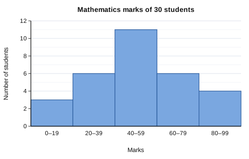
12.1.4Modal class and mean of grouped data

The modal class is the class with the highest frequency. For grouped data, the midpoint of a class = (lower limit + upper limit) ÷ 2. The mean is estimated by using the midpoint as the value of every item in the class. The mean of grouped data is written x̄ (read "x bar"), so x̄ = Σfx ÷ Σf.

Example 18 (textbook p. 259): modal class

Marks 40–44, 45–49, 50–54, 55–59, 60–64, 65–69 with frequencies 7, 4, 1, 4, 9, 5. The highest frequency is 9, so the modal class is 60–64.

Mean of grouped data (method of textbook Example 20, own numbers): time to walk to school, 24 students

Time (min)	Midpoint, x	Frequency, f	f × x
1–5	(1 + 5) ÷ 2 = 3	3	9
6–10	8	6	48
11–15	13	8	104
16–20	18	5	90
21–25	23	2	46
Total		24	297

Mean = Σfx ÷ Σf = 297 ÷ 24 = 12.4 minutes (1 d.p.). The modal class is 11–15.

Do not use the class limits (such as 11 or 15) in the calculation. Use the midpoint of each class. Σ means "the sum of", so Σfx is the total of the f × x column.

Find the modal class and the mean of: 0–4 (2 students), 5–9 (6), 10–14 (7), 15–19 (5).

Show answerHide answer

Modal class: 10–14 (frequency 7).
Midpoints 2, 7, 12, 17: Σfx = 4 + 42 + 84 + 85 = 215, Σf = 20.
Mean = 215 ÷ 20 = 10.75.

12.1.5Choosing the most appropriate measure

Measure	Use it when	Because
Mean	There is no extreme value	It uses every value in the set
Median	There is an extreme value	It is not affected by extreme values
Mode	The data is category data (not numbers), or you want the most popular item	You cannot add or order categories such as flavours

Example: monthly pay of 6 workers in a small shop (own numbers)

RM1 800, RM1 900, RM2 000, RM2 000, RM2 100, RM9 500 (the owner's son)
Mean = RM19 300 ÷ 6 = RM3 216.67, which is higher than five of the six workers earn. Median = RM2 000. The median describes this shop better, because RM9 500 is an extreme value.

Do not say "the mean is best because it is the average". Give a reason from the data: is there an extreme value, or is it category data?

12.1.6Mode, mean and median from data representations

Read the numbers carefully from a bar chart, dot plot, stem-and-leaf plot, pictograph or pie chart, and list them as a frequency table if you need to calculate.

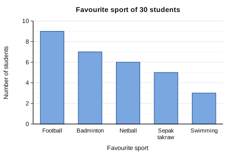
Bar chart of favourite sport of 30 students: football 9, badminton 7, netball 6, sepak takraw 5, swimming 3. — The tallest bar is football, so the mode is football. A bar chart of categories has no median or mean.

Bar chart / dot plot: bar height or number of dots is the frequency. Total frequency = number of data.
Pie chart: the largest sector is the mode. The median and mean of categories have no meaning.
Stem-and-leaf plot: read the key first. If 2 | 3 means 23, read each leaf with its stem. When the leaves are in order, count to the middle value.

Example 23 (textbook p. 265): a bar chart as a frequency table

Commissions RM30, 31, 32, 33, 34, 35 with frequencies 4, 5, 9, 7, 4, 1 (total 30).
Mean = (120 + 155 + 288 + 231 + 136 + 35) ÷ 30 = 965 ÷ 30 = RM32.17. Median = average of the 15th and 16th values = RM32. Mode = RM32.

Example 24 (textbook p. 265): find an unknown frequency

Number of spelling errors 0, 1, 2, 3, 4, 5 with frequencies 4, 8, x, 6, 5, 4, and mean 2.4.
(0 + 8 + 2x + 18 + 20 + 20) ÷ (27 + x) = 2.4, so 2x + 66 = 2.4(x + 27) = 2.4x + 64.8.
0.4x = 1.2, so x = 3.

An unknown value: write the mean formula with the unknown, multiply both sides by the total frequency, then solve the linear equation.

12.1.7Predictions, arguments and conclusions

To compare two groups or to choose between two people, the mean, median or mode may not be enough. The range (largest value − smallest value) shows how spread out the data is.

Example 25 (textbook p. 266): choosing a bowler

Ramesh: 116, 118, 200, 207, 209. Mean = 850 ÷ 5 = 170. Range = 209 − 116 = 93.
Khairil: 240, 240, 75, 220, 75. Mean = 850 ÷ 5 = 170. Range = 240 − 75 = 165.
The means are equal, so the mean cannot decide. Ramesh's scores are closer together (range 93, against 165), so he is more consistent and is the better choice.

Example 26 (textbook p. 267): which measure decides?

Goals scored by three teams in five competitions. Kijang: 65, 95, 32, 96, 88. Harimau: 50, 90, 65, 87, 87. Seladang: 90, 85, 46, 44, 80.
Means: Kijang 376 ÷ 5 = 75.2, Harimau 379 ÷ 5 = 75.8, Seladang 345 ÷ 5 = 69. By the mean, Harimau is best.
Medians: Kijang 88, Harimau 87, Seladang 80. By the median, Kijang is best.
The decision depends on the measure used. There is no extreme value, so the mean, which uses every value, is the most appropriate to report overall achievement.

A good conclusion has three parts: the value you calculated, the comparison, and the decision with a reason.

Summary

Idea	Key fact	Example
Mode	Value with the highest frequency; may be none or two	2, 3, 3, 5, 5, 7: modes 3 and 5
Median	Middle of ordered data; even n: average of two middle values	3, 5, 7, 9: (5 + 7) ÷ 2 = 6
Mean	Sum ÷ number; frequency table: Σ(value × frequency) ÷ Σf	2, 4, 9: 15 ÷ 3 = 5
Extreme value	Changes the mean, not the median or mode	5, 6, 7, 7, 8, 9, 20
Changing the data	Uniform change: all three change in the same way	All values × 3: mean × 3
Grouped data	Modal class = highest frequency; mean from midpoints, Σfx ÷ Σf	Class 11–15 has midpoint 13
Choosing a measure	Mean (no extreme value), median (extreme value), mode (categories)	Salaries: median
Range	Largest − smallest; shows consistency	93 against 165