Linear Law
What this chapter covers
- Differentiate between linear and non-linear relations from tables of data and graphs (6.1.1)
- Draw lines of best fit for graphs of linear relations, using suitable scales (6.1.2)
- Form the equation of a line of best fit, Y = mX + c, from two points or from the graph (6.1.3)
- Interpret information from a line of best fit, by reading the graph or by using its equation (6.1.4)
- Convert non-linear equations to the linear form Y = mX + c and identify Y, X, m and c (6.2.1)
- Use linear law to find unknown constants of a non-linear relation from a straight line graph (6.2.1)
- Solve problems that involve linear law, including logarithmic forms (6.3.1)
6.1Linear and non-linear relations
In Y = mX + c, X is the variable on the horizontal axis, Y is the variable on the vertical axis, m is the gradient and c is the Y-intercept.
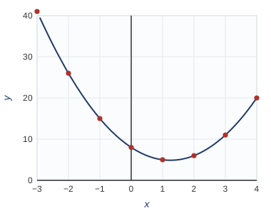
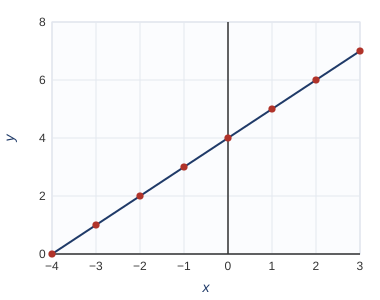
Y = X² gives Y = 1, 0, 1, 4 for the same X. The change in Y is not constant, so the graph is a curve: non-linear.
Show answerHide answer
Line of best fit
- Choose scales so the points fill most of the graph paper. Use a uniform scale such as 1 cm to 1 unit or 2 cm to 5 units.
- Draw with a ruler; do not join the points one by one.
- A point that is far from the trend, for example one recorded wrongly, is marked and left out, as the line follows the trend of the rest (see Intensive Practice 6.3, Q2 on p. 168).
Equation of a line of best fit
Choose two points on the line (not data points that are off the line), then find m = (Y₂ − Y₁) ÷ (X₂ − X₁) and c from the Y-intercept, or by substituting one point into Y = mX + c.
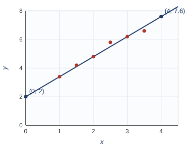
Equation: y = 1.4x + 2.
Interpreting the graph
Use the line (or its equation) to find values that were not measured. Reading from the line within the plotted values is interpolating; extending the line beyond is extrapolating. The equation is more accurate than reading the graph.
When x = 0: log₁₀ y = 0.2, so y = 100.2 = 1.585.
When y = 20: log₁₀ 20 = 1.3, so 2x + 0.2 = 1.3 and x = 0.55.
Show answerHide answer
y = 12: 1.4x = 10, so x = 7.14.
6.2Linear law and non-linear relations
Converting to the linear form
| Non-linear equation | Step | Y | X | m | c |
|---|---|---|---|---|---|
| y = ax² + b | already linear in x² | y | x² | a | b |
| y = ax + b/x | multiply by x: xy = ax² + b | xy | x² | a | b |
| y = ax + b/x | divide by x: y/x = b(1/x²) + a | y/x | 1/x² | b | a |
| y = px² + qx | divide by x: y/x = px + q | y/x | x | p | q |
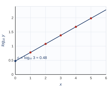
| y = pqx | take log₁₀: log y = (log q)x + log p | log₁₀ y | x | log₁₀ q | log₁₀ p |
| y = axb | take log₁₀: log y = b log x + log a | log₁₀ y | log₁₀ x | b | log₁₀ a |
From the line: Y-intercept = 22 and gradient = −2.
q/3 = 22, so q = 66. p/3 = −2, so p = −6.
Show answerHide answer
Second: log₁₀ y = k log₁₀ x + log₁₀ h. Y = log₁₀ y, X = log₁₀ x, m = k, c = log₁₀ h.
6.3Applications of linear law
Follow the textbook's four steps for a problem: understand (what are the variables and the axes), plan (convert to Y = mX + c, make a new table), implement (plot, read m and c, find the constants), conclude (check by substituting back).
So Y = (P − 180)/K, X = K, m = −s, c = r.
From the graph: c = 1.6, so r = 1.6; gradient −s = −0.56, so s = 0.56.
Check with K = 3: P = 180 + 1.6(3) − 0.56(9) = 179.76, matching the table (179.7).
Show answerHide answer
Notes follow Additional Mathematics Form 4 KSSM (DLP), Chapter 6, pp. 152 to 173; figures are redrawn from the textbook examples.