Measures of Dispersion for Ungrouped Data
What this chapter covers
- Explain the meaning of dispersion (8.1.1)
- Compare and interpret the dispersion of two or more sets of data using stem-and-leaf plots and dot plots, and draw a conclusion (8.1.2)
- Find the range, interquartile range, variance and standard deviation of ungrouped data, including data in a frequency table (8.2.1)
- Explain the advantages and disadvantages of the measures of dispersion (8.2.2)
- Construct and interpret a box plot for ungrouped data (8.2.3)
- Determine the effect on the measures of dispersion when the data is changed by adding, multiplying, or by an outlier or removed value (8.2.4)
- Compare sets of ungrouped data using suitable measures of dispersion and solve problems involving measures of dispersion (8.2.5, 8.2.6)
8.1Dispersion
The simplest way to see dispersion is the difference between the largest and the smallest value. Range, interquartile range, variance and standard deviation are the measures of dispersion you will use in this chapter.
Difference = 79 kg − 47 kg = 32 kg. A bigger difference means the data is more widely dispersed.
Dot plots and stem-and-leaf plots
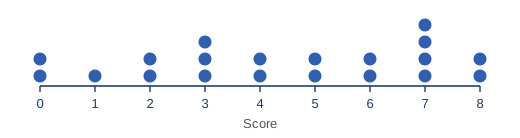
A dot plot puts one dot above a number line for each value, so repeated values pile up. It suits a small set of data. A stem-and-leaf plot splits each value into a stem (the tens) and a leaf (the units). Leaves are written in order, smallest first, and a key is always given.
| Stem | Leaf |
|---|---|
| 2 | 7 9 |
| 3 | 1 2 4 5 5 6 7 7 8 8 9 |
| 4 | 0 0 1 2 2 2 2 3 4 4 5 6 7 7 7 8 9 9 |
| 5 | 2 2 2 3 4 |
Key: 2 | 7 means 27 marks. Accounting test marks of 36 pupils, textbook p. 215. Most marks are in the 40s.
(a) The Science scores are more dispersed because their difference is larger.
(b) The Mathematics scores are better because most of its dots are on the right.
Show answerHide answer
8.2Measures of dispersion
Range
From a frequency table, take the smallest and largest values of x that have a frequency. Do not subtract frequencies.
Frequency table with scores 2 to 8: range = 8 − 2 = 6.
Interquartile range
- Arrange the data in ascending order and find the median.
- Split the data into a part before the median and a part after it. If n is odd, the median itself is left out of both parts.
- Q1 is the median of the lower part and Q3 is the median of the upper part. With an even number of values, take the average of the two middle values.
- Interquartile range = Q3 − Q1.
(b) 11, 14, 14, 17, 19, 20, 20, 21, 22 (n = 9). Median 19. Q1 = 14+142 = 14, Q3 = 20+212 = 20.5. IQR = 6.5.
From a frequency table
Add a cumulative frequency row. Q1 is the value at position 14N and Q3 is the value at position 34N.
| Score | 2 | 3 | 4 | 5 | 6 | 7 | 8 |
|---|---|---|---|---|---|---|---|
| Frequency | 3 | 5 | 6 | 8 | 12 | 7 | 3 |
| Cumulative | 3 | 8 | 14 | 22 | 34 | 41 | 44 |
Variance and standard deviation
| Data | Variance σ² | Standard deviation σ |
|---|---|---|
| Ungrouped list | Σ(x − x̄)²N = Σx²N − x̄² | √σ² |
| Frequency table | Σf(x − x̄)²Σf = Σfx²Σf − x̄² | √σ² |
The mean is x̄ = ΣxN, or ΣfxΣf for a frequency table. The shortcut with Σx² is usually quicker and needs fewer subtractions.
σ² = 4 + 16 + 25 + 25 + 365 − 4.4² = 21.2 − 19.36 = 1.84.
(b) Books read: 0, 1, 2, 3, 4 with frequencies 3, 5, 8, 2, 2 (Σf = 20).
Σfx = 35, so mean = 1.75. Σfx² = 87.
σ² = 8720 − 1.75² = 4.35 − 3.0625 = 1.2875.
σ = √1.2875 = 1.135.
Show answerHide answer
σ² = 198 ÷ 5 − 36 = 3.6. σ = √3.6 = 1.897.
Choosing a measure
| Measure | Advantage | Disadvantage |
|---|---|---|
| Range | Easiest to find | Only two values; badly affected by an outlier |
| Interquartile range | Not affected much by outliers | Ignores the lowest and highest quarter |
| Standard deviation | Uses every value; best for comparing sets | Pulled up by an outlier; more working |
Box plots
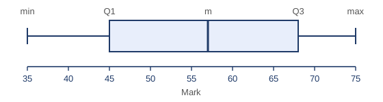
Show answerHide answer
Effect of changing the data
| Change to every value | Range | IQR | Standard deviation | Variance |
|---|---|---|---|---|
| Add or subtract k | same | same | same | same |
| Multiply by k | × k | × k | × k | × k² |
| Divide by k | ÷ k | ÷ k | ÷ k | ÷ k² |
When you do two steps, such as "multiply by 4, then add 2", the adding has no effect and only the multiplying counts.
New range = 25 × 4 = 100. New variance = 2.7 × 4² = 43.2.
Adding or removing a value
- An outlier added makes the range and the standard deviation much larger. The IQR changes little.
- A value added close to the mean makes the standard deviation smaller. A value far from the mean makes it larger.
- Removing a value far from the mean makes the standard deviation smaller.
Problems with Σx and Σx²
Σx = 936 + 672 = 1 608. Σx² = 48 717 + 37 653.6 = 86 370.6.
Combined mean = 1 608 ÷ 30 = 53.6.
σ² = 86 370.6 ÷ 30 − 53.6² = 6.06, so σ = 2.462.