Mathematics notes, chapter 8

Mathematical Modeling

Textbook Mathematics Form 5 (DLP), pages 226–243

What this chapter covers

Explain mathematical modeling, the difference between a closed problem and an open-ended problem, and the components of the modeling process (8.1.1)
Make assumptions, identify variables, verify, refine and report a model (8.1.2)
Solve real-life problems through mathematical modeling that involves linear, quadratic and exponential functions, choosing the function from the pattern of the data (8.1.2)
Build and use the compound interest model A(t) = P(1 + r/n)^nt and communicate the modeling process (8.1.2)

8.1aWhat is mathematical modeling?

A mathematical model is a mathematical relation that describes a real-world situation. It helps us understand the situation and predict future behaviour. Mathematical modeling is the process of building, using and improving such a model.

For example, I = Prt is a model that links simple interest, I, to the principal, P, the rate, r, and the time, t.

Closed problems and open-ended problems

	Problem solving question	Open-ended real-world problem
Information	All the information needed is given	Information is incomplete; we must find it or assume it
Answer	One correct answer	Several valid models and answers are possible
Example	40 000 people, 45% recycle, 5 bottles each a week: how many bottles?	How long does it take to clean up an oil spill in the ocean?

Modeling is meant for the right-hand column: problems that need mathematics and creativity.

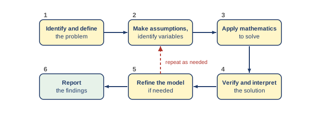
The six components of the modeling process

Flow chart: identify and define the problem, make assumptions and identify variables, apply mathematics, verify and interpret, refine the model, report the findings; refine loops back as needed — The modeling process (textbook p. 230). The model is refined and the cycle repeated as often as needed.

Component	What you do
1. Identify and define the problem	State what is to be found; list the information needed and where to get it
2. Make assumptions and identify the variables	Simplify the situation; give each quantity a letter (a variable is a quantity with an unknown value)
3. Apply mathematics	Build the model (an equation, inequality, table or graph) and calculate
4. Verify and interpret	Does the answer solve the problem? Is it sensible in the real world?
5. Refine the model	Change assumptions that are unrealistic, then repeat
6. Report the findings	Use symbols and diagrams; state the strengths and weaknesses of the model

Treating the worked example as a template. The textbook stresses that its example is not a template: different people may build different valid models and reach different answers.

Worked model: is it worth driving to the cheaper rice store?

Textbook pp. 230-233: store A is near, store B is cheaper but farther

Assumptions: the route is a straight line; the same number and brand of rice is bought at both stores.
Variables: P₁, P₂ = price of a 10 kg pack at stores A and B (RM); n = number of packs; s = extra distance to store B (km); m = petrol consumption (km per litre); H = petrol price (RM per litre).
Model:
Saving on rice, S = (P₁ − P₂) × n
Extra petrol cost, T = sm × H × 2 (× 2 for the return trip)
If S > T it is sensible to drive to store B. If S < T it is not.

Using it: P₁ = 25.95, P₂ = 23.99, n = 2, s = 6, m = 17.6, H = 2.08
S = (25.95 − 23.99) × 2 = RM3.92 T = 617.6 × 2.08 × 2 = RM1.42
S > T, so you save RM3.92 − RM1.42 = RM2.50 by driving to store B.

A good model also answers other questions. With the same numbers, store B is worth the trip only if s < 16.6 km (from S > T), and only if P₂ < RM25.24.

Reflecting, refining and reporting

Reflect: Are the assumptions reasonable? What if they are wrong? Does the answer change a lot if an input changes a little?
Refine: If the route is not a straight line (for example store A is 2 km from the house and store B is 4 km from store A, at a right angle, so the extra distance is not simply 4 km), the assumption must be changed and the model revised.
Report: state limitations. This model ignores the value of the driver's time and the effect on the environment.

State two assumptions you would make to model "Will it be cheaper to cook at home than to buy lunch for a week?"

Show answerHide answer

Any two sensible assumptions, for example: prices of ingredients and food stay the same for the week; the same number of meals is eaten each day; the cost of gas and electricity is ignored (or is a fixed amount); no food is wasted.

Example 1 (textbook p. 234): Jeremy saves RM4 000 at 1.5% simple interest per annum to buy a RM4 455 computer. How long must he save?

(a) Problem: the interest needed is RM4 455 − RM4 000 = RM455; find the time in years.
(b) Assumptions: the interest rate does not change (otherwise I = Prt is not suitable); the price of the computer does not change.
Variables: I = interest, P = principal, r = rate, t = time in years.

Continue Example 1: use I = Prt to find how long Jeremy must save.

Show answerHide answer

I = 455, P = 4 000, r = 0.015
455 = 4 000 × 0.015 × t = 60t
t = 455 ÷ 60 ≈ 7.6, so he needs 8 years (the interest is only credited each full year).

8.1bSolving problems with linear, quadratic and exponential models

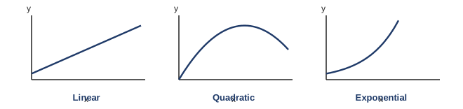
Choosing the type of function from the graph

Three graphs: a rising straight line labelled linear, a parabola labelled quadratic, a curve that rises ever faster labelled exponential — Study the pattern of the data points to choose the model (textbook p. 236).

Model	Shape of the graph	Form	Typical situation
Linear	Straight line	y = mx + c; y = kx for direct variation	Petrol used and distance, with constant rate
Quadratic	Parabola: rises then falls, or falls then rises	y = ax² + bx + c	Depth of a river, path of a ball
Exponential	Curve that increases or decreases at a sharp rate	y = Ca^x, a > 0, a ≠ 1, C = initial value	Compound interest, population growth

Each model is only valid for a stated range of the variables. Never extend a model far beyond its data without checking.

Linear model (Example 2, textbook p. 236)

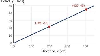
Amin travelled 405 km on 45 litres. How much petrol for 198 km?

Assumption: the driving speed is the same on both routes. Variables: x = distance (km), y = petrol (litres), y varies directly with x, so y = kx.
Solve: 45 = k(405), k = 45405 = 19, so y = 19x.
x = 198: y = 19 × 198 = 22 litres.
Verify: if the 405 km route is through towns and the 198 km route is on a highway, the car uses petrol at different rates, so the linear model does not suit the situation.

Straight line through the origin passing through (198, 22) and (405, 45) — y = x/9 passes through the origin: direct variation.

A van uses 36 litres for 450 km. Assuming y = kx, find the petrol needed for 275 km.

Show answerHide answer

36 = k(450), k = 0.08
y = 0.08 × 275 = 22 litres

Quadratic model (Example 3, textbook pp. 237-238)

River depth, y m, at distance x m from the bank

x	0	4	8	12	18	25	30
y	0	1.5	2.3	2.9	2.9	1.7	0

The points rise and then fall, like a parabola, so use y = ax² + bx + c.
Substitute (0, 0): c = 0.
Substitute (25, 1.7): 1.7 = 625a + 25b (1)
Substitute (30, 0): 0 = 900a + 30b, so b = −30a (2)
Put (2) in (1): 1.7 = 625a − 750a = −125a, so a = −0.0136 and b = 0.408.
Model: y = −0.0136x² + 0.408x
Check: x = 15 gives y = −0.0136(225) + 0.408(15) = 3.06, close to the 3 m read from the graph.

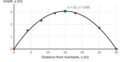
Seven data points of river depth with a parabola through them, highest near x = 15 — The fitted curve and the data. The assumption that the river is deepest in the middle may not be true for other rivers.

Any three points that are on the curve will give a quadratic. Choose points whose substitution is easy, such as the one where x = 0. More data makes the model more accurate.

Forgetting that c = 0 when the curve passes through the origin, so the system has three unknowns instead of two. Always use (0, 0) first if it is in the data.

Exponential model (Example 4, textbook pp. 239-240)

Compound interest: RM20 000 at 4% per annum, compounded once a year

Year	Amount at the end of the year (RM)
1	20 000(1.04)
2	20 000(1.04)²
3	20 000(1.04)³
5	20 000(1.04)⁵ = 24 333.06

Each year the amount is multiplied by 1.04 = 1 + r. The pattern gives the model
A(t) = P(1 + r)^t

Curve of A(t) = 20 000 times 1.04 to the power t, rising slowly then faster up to about 96 000 at 40 years — Exponential growth: the amount increases faster as time goes on.

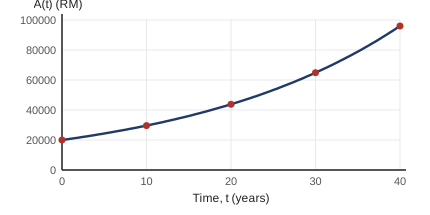
If interest is compounded n times a year, the rate per period is r/n and there are nt periods:
A(t) = P(1 + rn)^nt

Compounded	n	A(t)
Annually	1	P(1 + r)^t
Semi-annually	2	P(1 + r/2)^2t
Quarterly	4	P(1 + r/4)^4t
Monthly	12	P(1 + r/12)^12t

Using the full rate r for each period, or forgetting to multiply t by n. For 8% compounded quarterly use 2% per period and 4t periods.

RM8 000 is saved at 6% per annum compounded quarterly for 2 years. Find the amount.

Show answerHide answer

Rate per period = 6% ÷ 4 = 1.5%; periods = 4 × 2 = 8
A = 8 000(1.015)⁸ = RM9 011.94

Reporting the findings

Write the full report using the six components: problem, assumptions and variables, mathematics, verification, refinement, then the conclusion with the model's strengths and weaknesses.